[B-Rep Generation] HoLa: B-Rep Generation using a Holistic Latent Representation

[B-Rep Generation] HoLa: B-Rep Generation using a Holistic Latent Representation

• paper: https://arxiv.org/pdf/2504.14257
• github: X
• ACM TOG 2025 & SIGGRAPH 2025 accpeted (인용수: 2회, ‘25-09-27 기준)
• Downstream task: 3D CAD B-REP (Boundary Representation)을 생성하는 task (Conditional / Unconditional)

1. Motivation

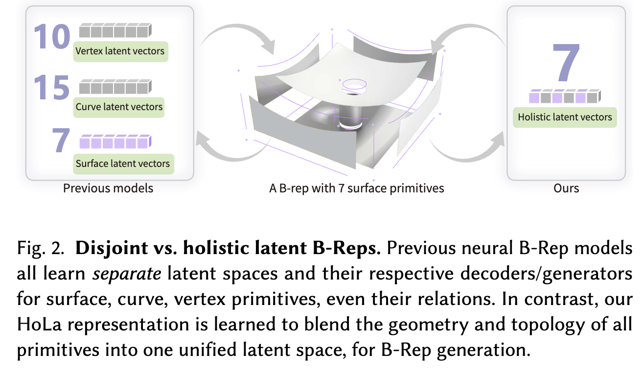
• 기존 연구들에서는 3D 물체의 표면, 경계 곡선, 그리고 topological 관계를 서로 다른 표현공간 (representation space) encoding하여 학습하였음.

  • 한계점
    • 명시적인 (Explicit) topological 제약이 없었기에 표면 $\to$ 곡선 multi step으로 생성 할 때 error accumulation 발생

  $\to$ 인접하는 표면간에 접선이 경계곡선으로 표현되는 사전 지식 (inductive bias)를 바탕으로, 통합된 표현공간으로 encoding해보면 어떨까?

  

2. Contribution

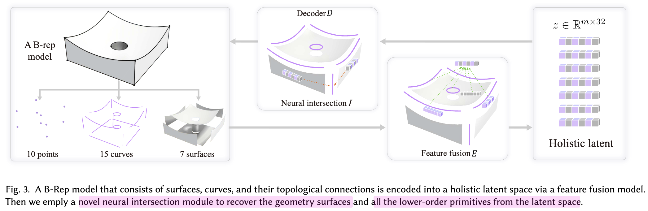
• 3차원 표면 pair 간의 연결성을 (intersection) module을 통해 연결유무를 파악하고, 표면 & 곡선 정보를 통합된 latent로부터 복원하는 Holistic Latent (HoLa)를 제안함.

  

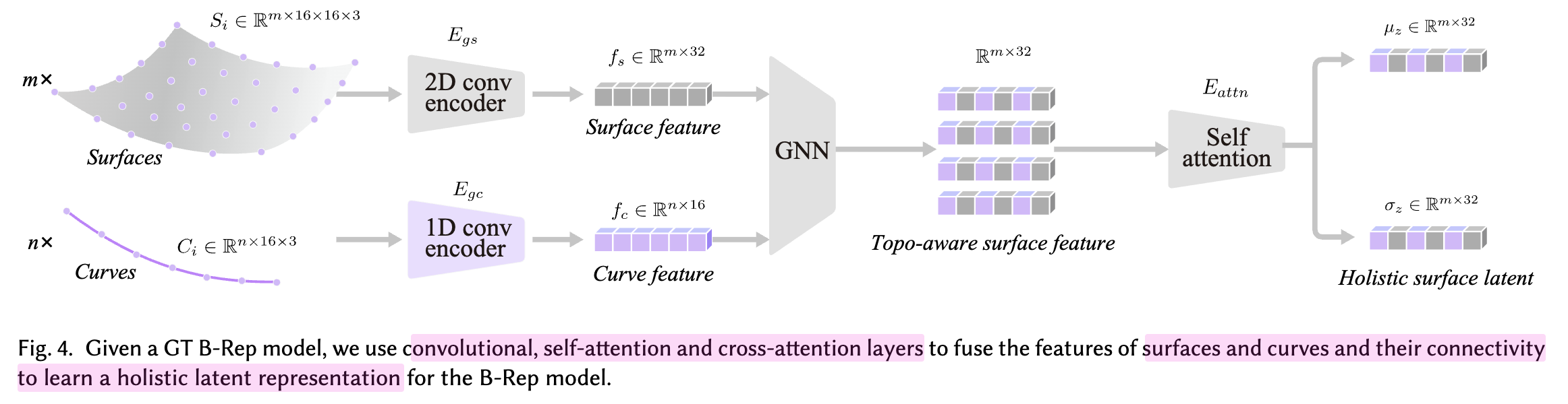
  • VAE (conv + self-attention + cross-attention)
    • input: curves / surfaces
    • output: latent vector $z$
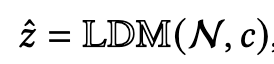
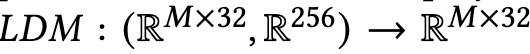
  • Latent Diffusion Model (LDM)
    • input
      • condition vector ($c \in R^{256}$)
      • latent vector $z$
    • output
      • curves
      • surfaces

3. HoLa

Overview

• CAD Model
  • $S$: Surface. ${S_i}_{i=1}^m$
    • B-Spline로 표현하며, uniform sampling을 통해 ($16\times16\times3$)로 정의
  • $C$: Curve. ${C_i}_{i=1}^n$
    • B-Spline로 표현하며, uniform sampling을 통해 ($16\times3$)로 정의
  • $V$: Vertices. ${V_k}_{k=1}^l$
  • $T_{SC}$: Surface-to-Curve connections $\in {0, 1}, R^{m \times n}$
    • ${V, T_{sc}}$를 통해 Vertice를 curve에 묶어서 표현
  • $T_{CV}$: Curve-to-Vertices connections $\in {0, 1}, R^{n \times l}$

• VAE Training

  • encoder

    

    • input: ${S,C,T_{SC}}$

      

      

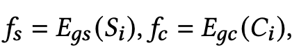
      • Downsample + CNN: $S \in R^{m \times 16 \times 16 \times 3} \to R^{m \times 32}$
      • Downsample + CNN: $C \in R^{n \times 16 \times 3} \to R^{n \times 16}$
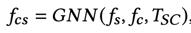
      • GNN: $(R^{m \times 32}, R^{n \times 16}, {0,1}^{m \times n}) \to T_{SC} \in R^{m \times n}$: curve-aware feature vector ($f_{sc}$)
      • Self-attention layer: $R^{m \times n} \to R^{m \times n}$
      • MLP layer: $E_{mlp}: R^{m \times n} \to (R^{m \times n}, R^{m \times n})$

    • output: $z_s \in R^{m \times (2\times2\times d)}$

      • m: surface별 embedding
      • 2: spatial resolution
      • 2: direction
      • d = 8 : feature dimension

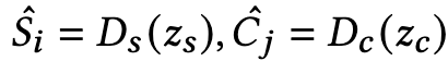
  • decoder:

    

    • input: : $z_s \in R^{m \times (2\times2\times d)}$

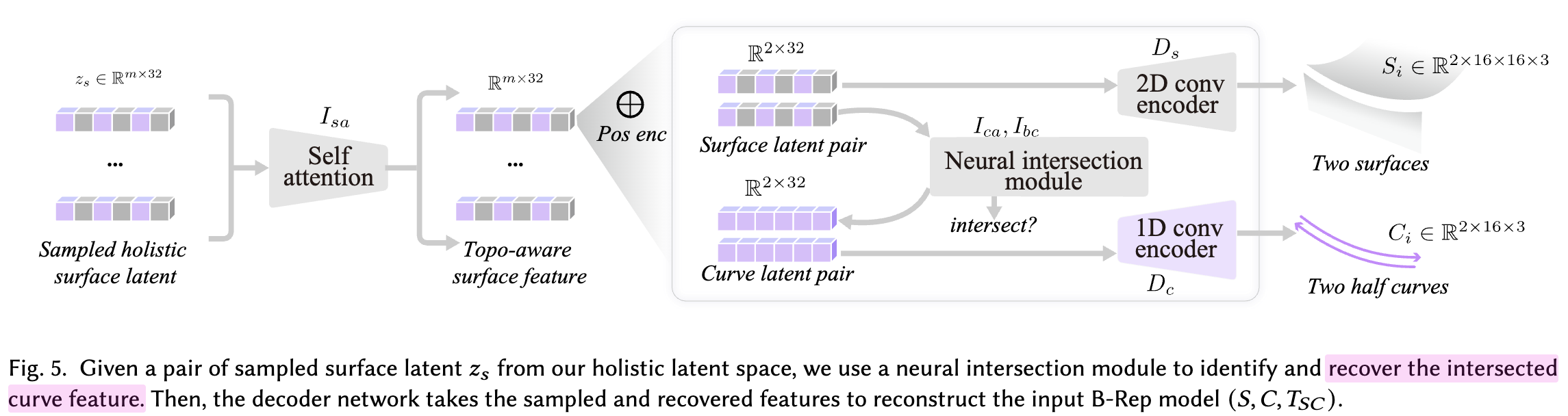
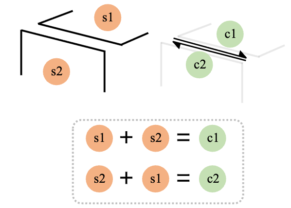
    • intersection Module $\mathbb{I}: R^{(m \times 32, m \times 32)} \to (R^{16}, {0,1})$

      • curves, vertices 를 latent space에 반영하게 하기 위해 사용
        • Self-attention + cross-attention + MLP 통과
          • self-attention: $R^{32} \to R^{32}$
          • cross-attention: $(R^{32}, R^{32}) \to R^{16}$
          • mlp: $R^{16} \to R^{16}$
          • binary classifier: $R^{16} \to {0,1}$
        • surface가 몇번째인지 positional encoding 정보 추가
      • input: m개의 surface latent 쌍
      • output: 두 surface가 접하는지 (1) 아닌지 (0) 예측

    • output: ${S,C,T_{SC}}$

      

      

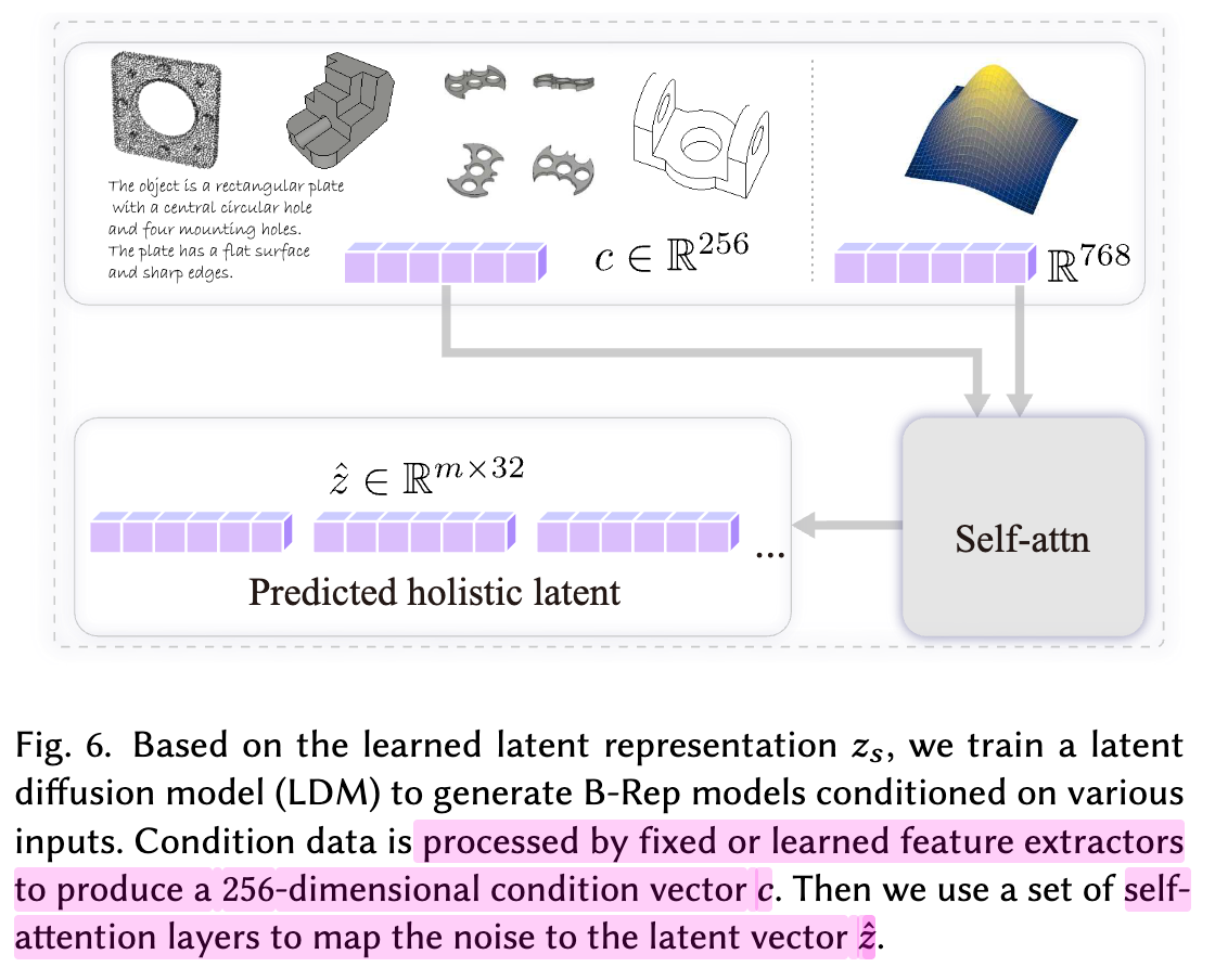
• LDM Training

  • input
    • Conditions: $c \in R^{256}$
    • Latent embedding $z_s \in R^{m \times (2\times2\times d)}$
  • Output: ${S,C,T_{SC}}$

• Loss

  

  

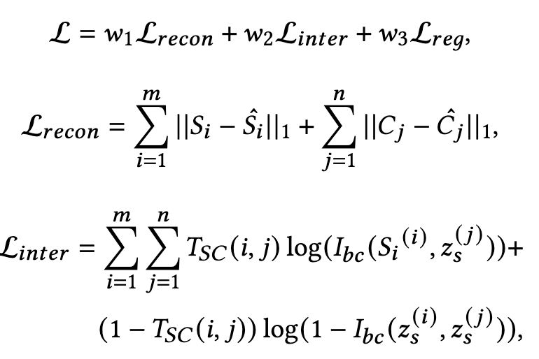
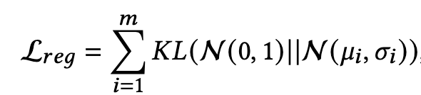
• Half-Curvature

  

  • $16 \times 3$로 curve를 uniform sampling하는 과정에서 curve의 방향이 고정되어, 임의로 방향이 지정됨 $\to$ 이는 학습을 robust하지 못하게 함
  • L1 loss대신 Chamfer distance 을 적용 (inner hole: clock-wise loop, outer hole: counter-clock wise)

• (Conditional) Generation

  

  • condition을 latent와 함께 부여하여 복원

    

    

    • image: dinov2 embedding (1024d) $\to$ MLP (256d)
      • 학습할 때 freeze
    • point clouds: PointNet
      • 학습할때 unfreeze

• Post-process

  • Intersection module + Decoder 통과 후, embedding은 BSpline을 통해 sample points를 surface, curves로 복원

4. Experiments

• Dataset
  • DeepCAD dataset
    • 7 ~ 30 surfaces를 갖는 models만 활용
      • Train: 47,284
      • val: 3,517
      • test: 2,424
• Evaluation Metrics
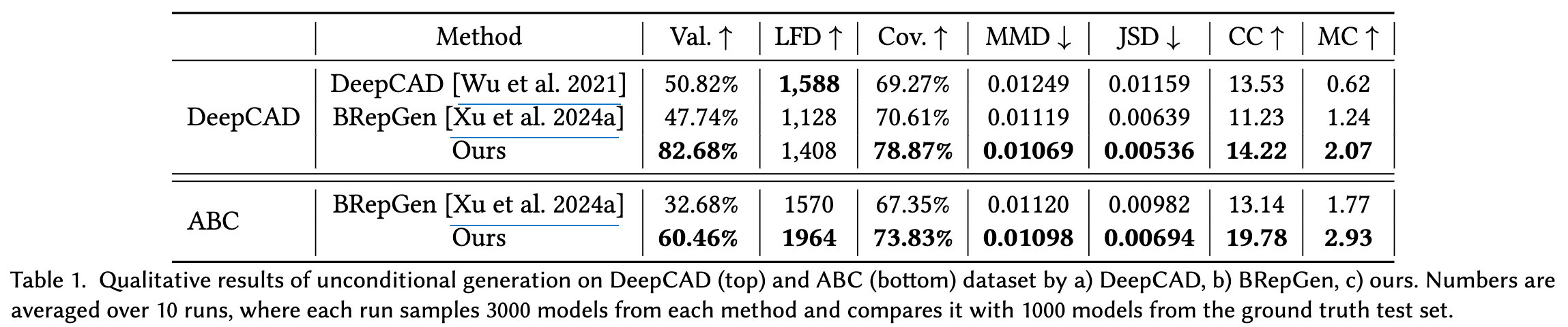
  • Validity ($\uparrow$): 전체 생성된 samples중 유효한 samples의 비율
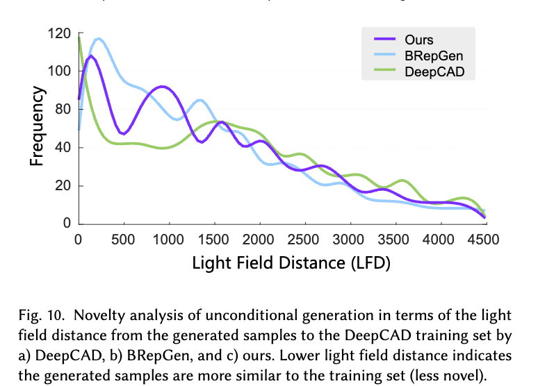
  • Average Light Field Distance (LFD) ($\uparrow$): light field distance를 기반으로 생성된 sample의 “novelty”를 평가함. 얼마나 training set 기준 overfitting이 덜되었는지 평가
  • Coverage ($\uparrow$): 생성된 samples로 cover되는 test-set의 비율. Chamfer Distance (CD)기반으로 closest neighbor를 선정
  • Jensen-Shannon Divergence (JSD) ($\downarrow$): 생성된 samples와 test set의 분포 차이 ($28^3$ voxel point cloud로 표현)
  • Maximum-Mean Discrepancy (MMD) ($\downarrow$): 생성된 sample과 nearest neighbor로 mapping된 test-set의 평균 CD 거리
  • Cyclomatic Complexity (CC) ($\uparrow$): 생성된 sample의 wireframe graph 표현 에 존재하는 loop의 수. 복잡도를 표현
  • Mean curvature (MC) ($\uparrow$): 생성된 samples의 averaged mean curvature

• 정량적 결과

  

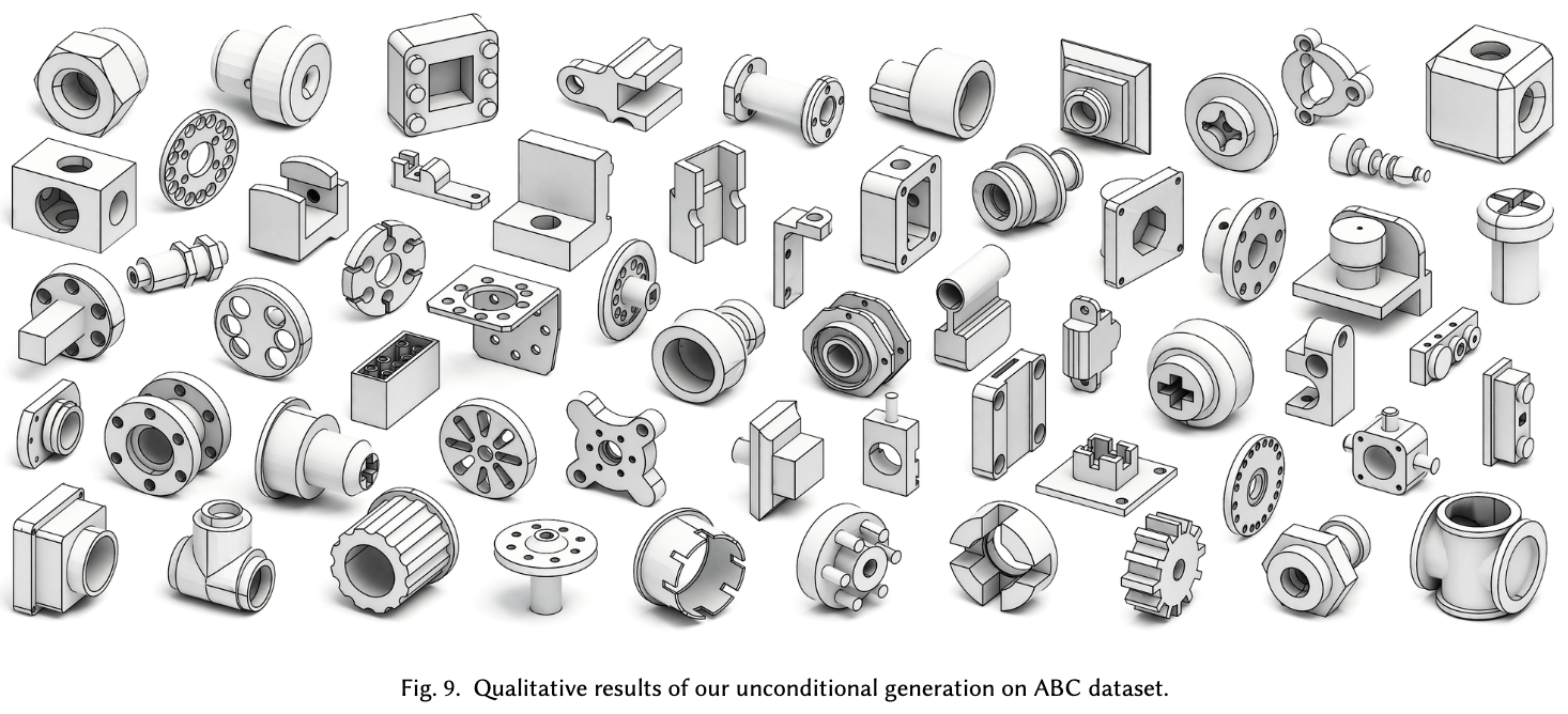
• 정성적 결과

  

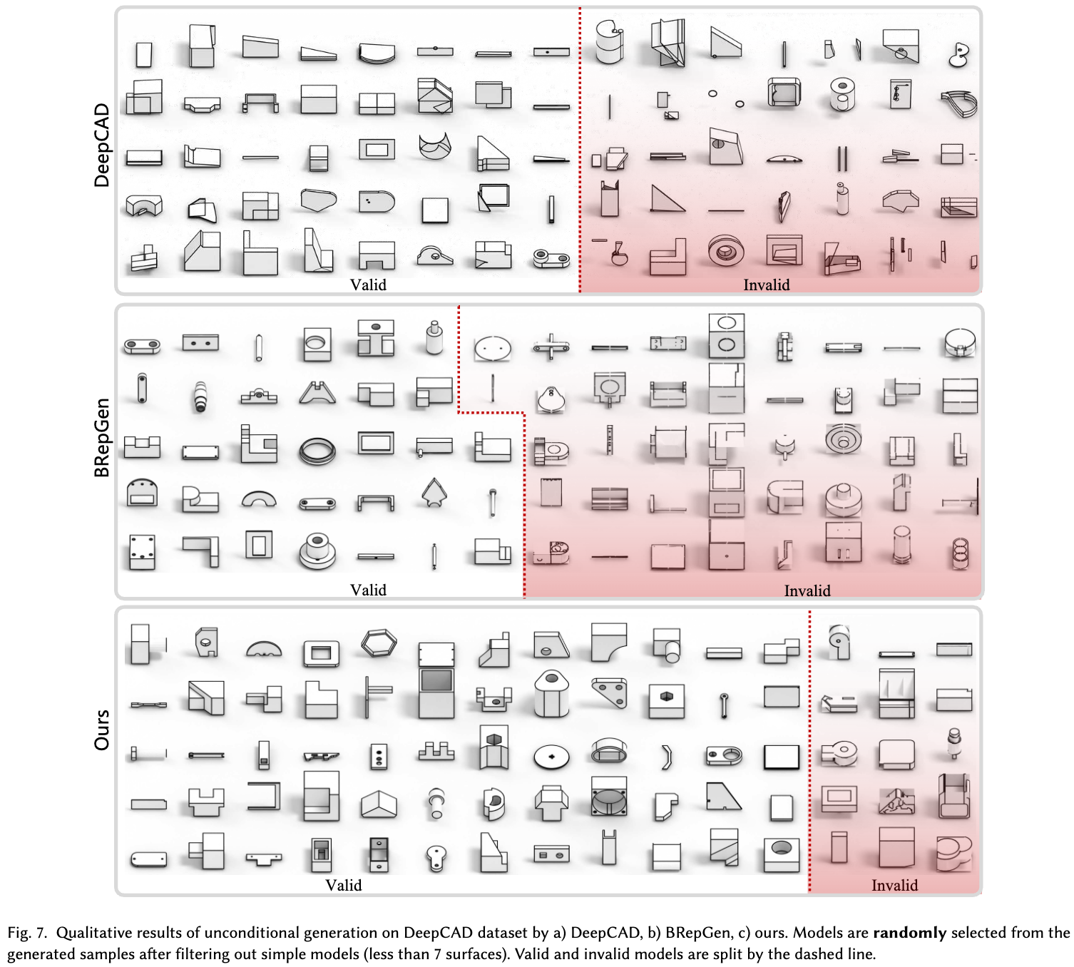
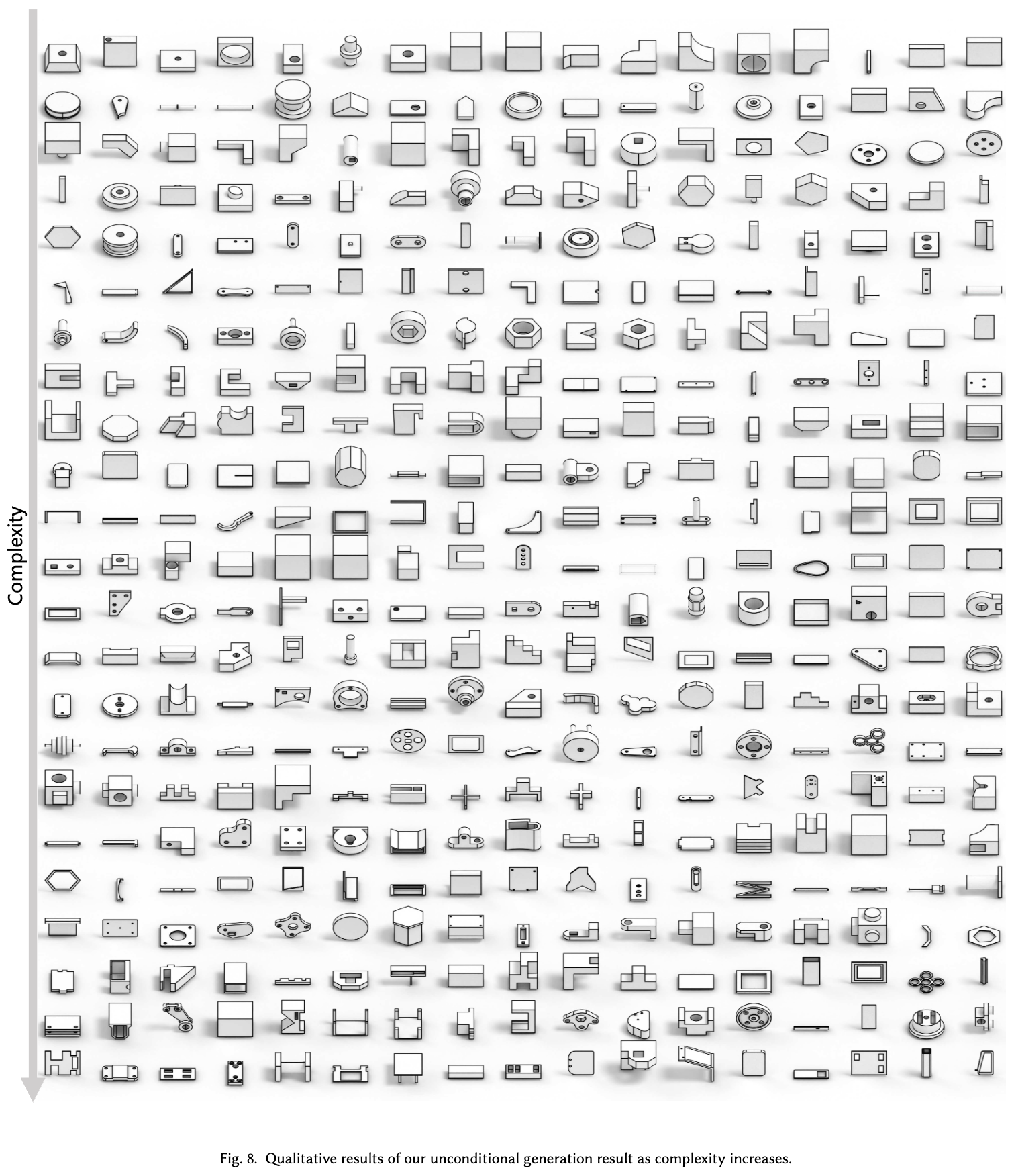
• Unconditional Generation 결과

  

  

  

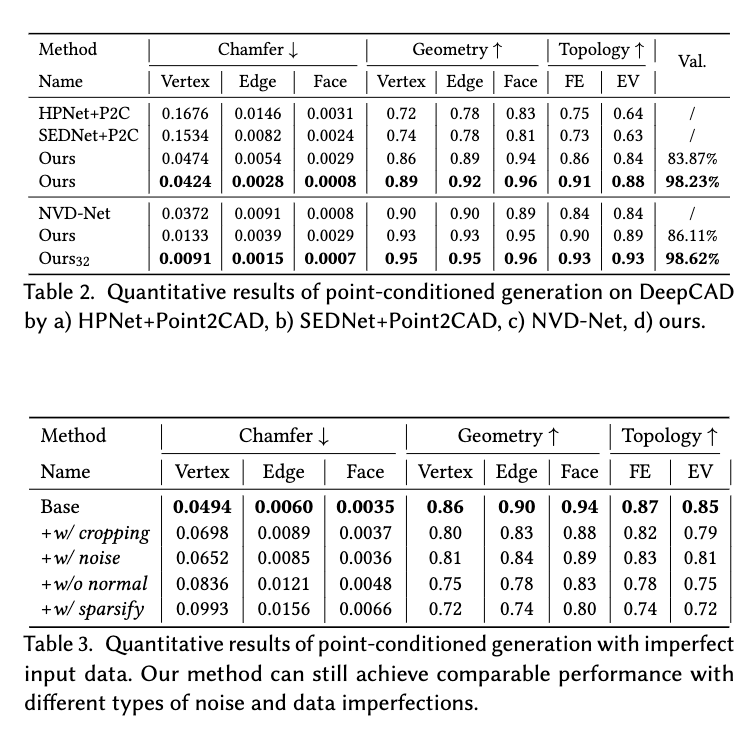
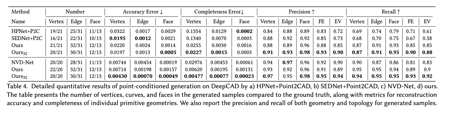
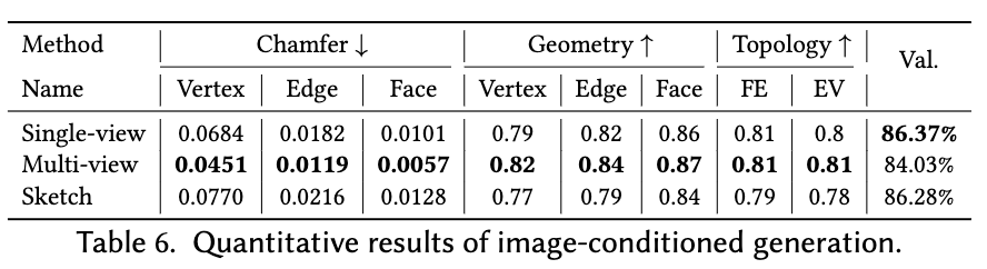
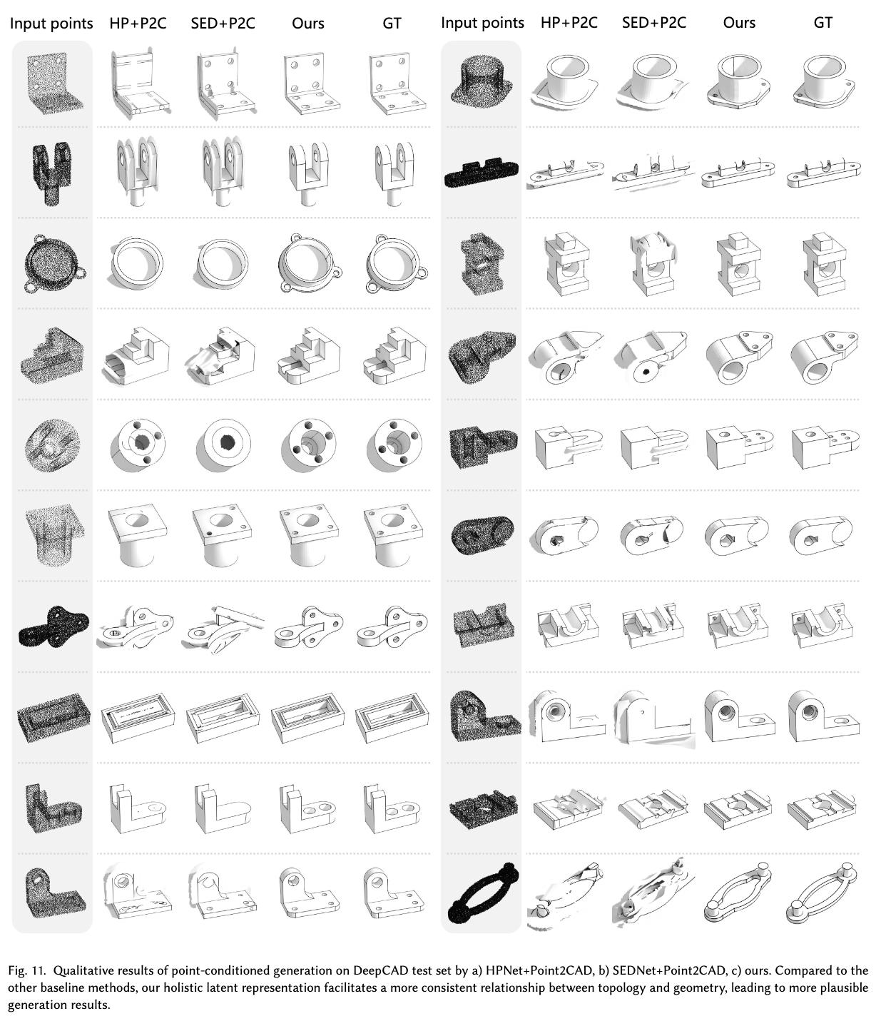
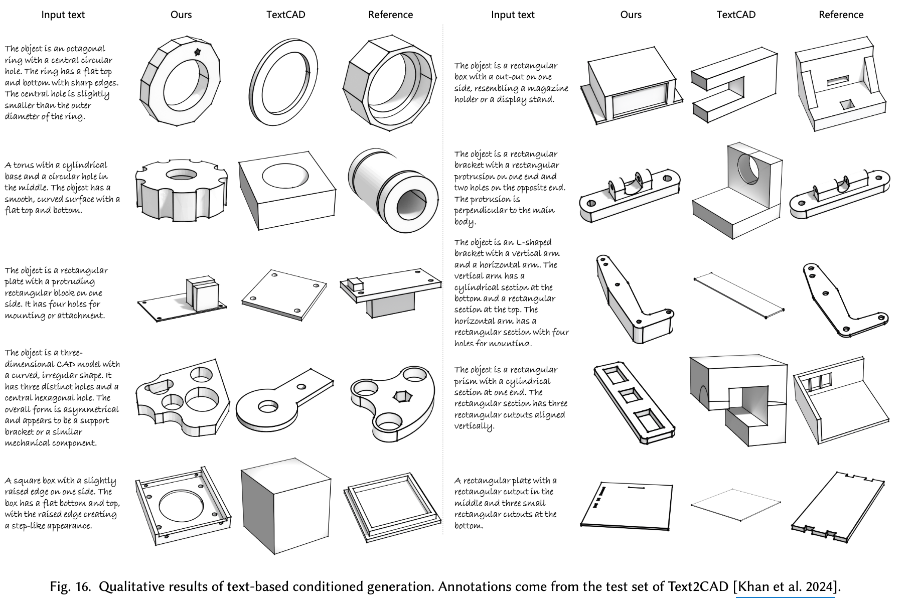
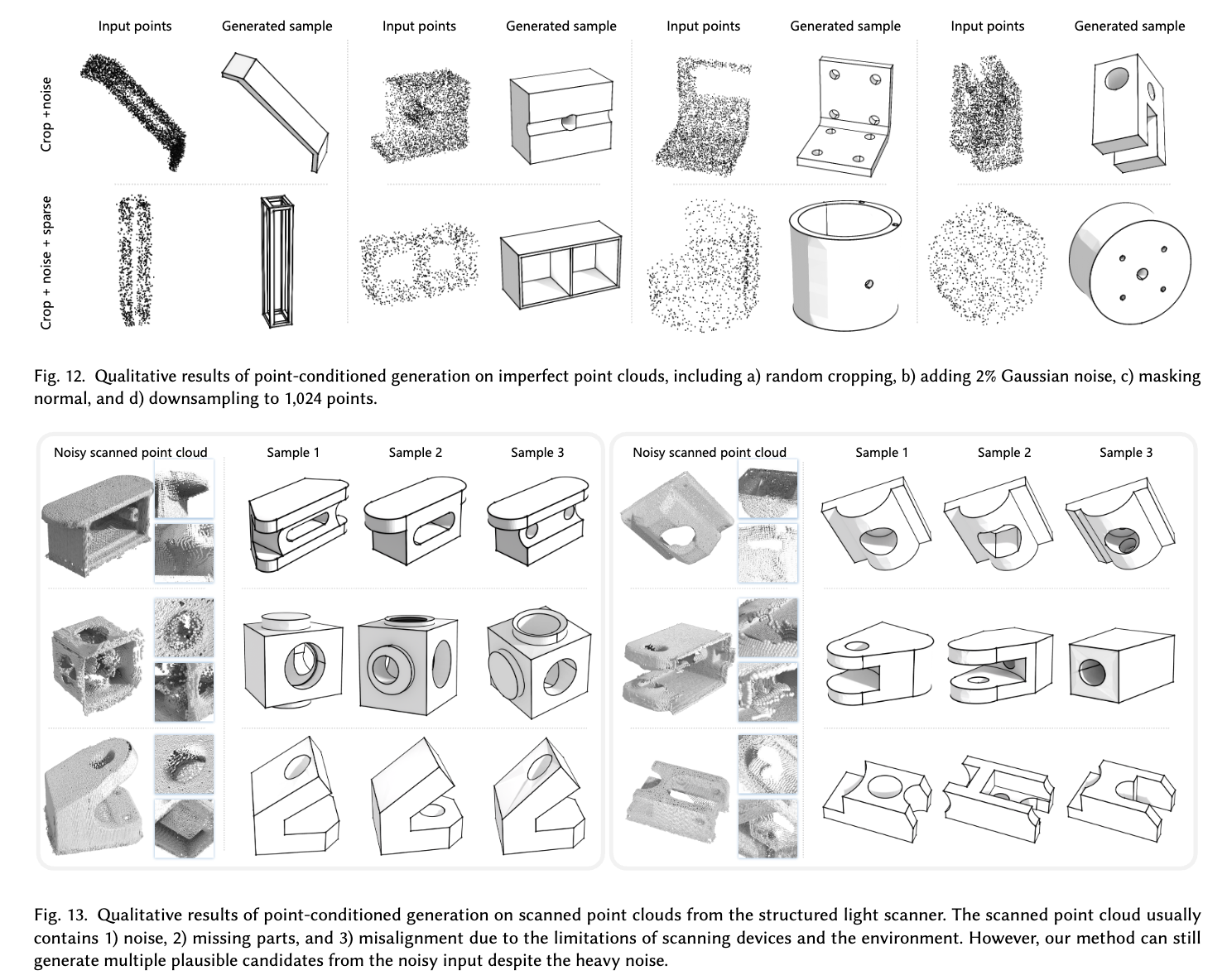
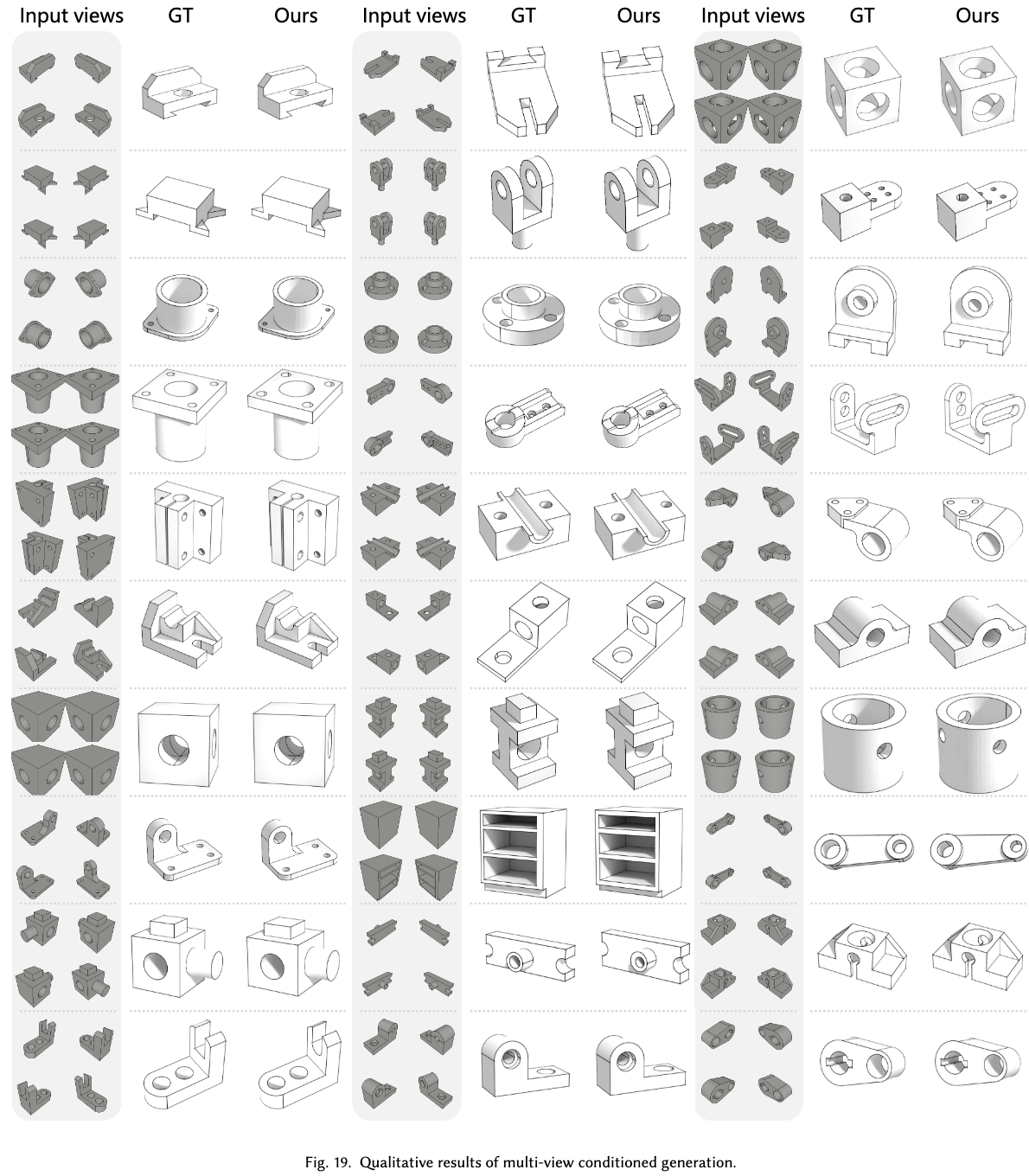
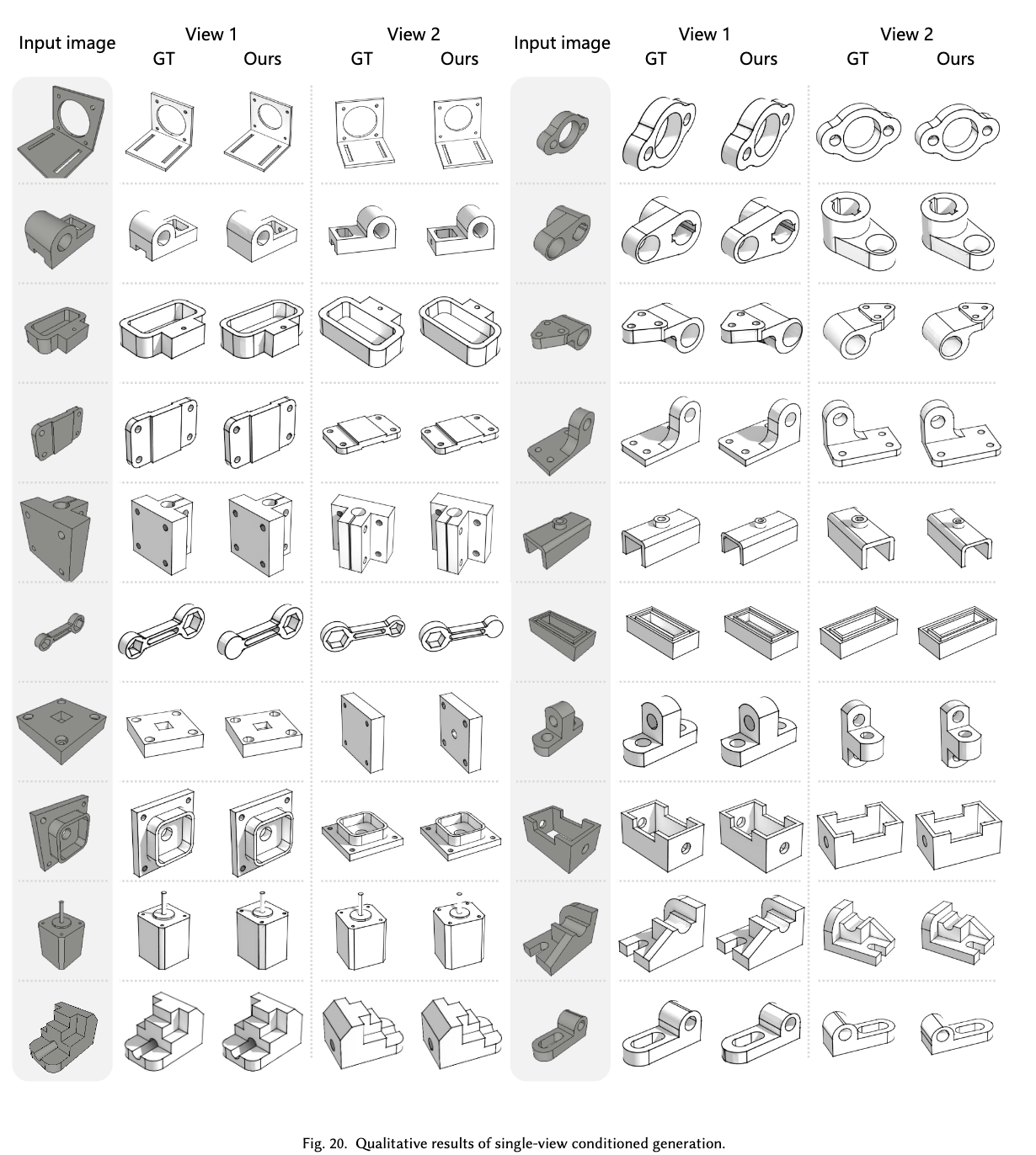
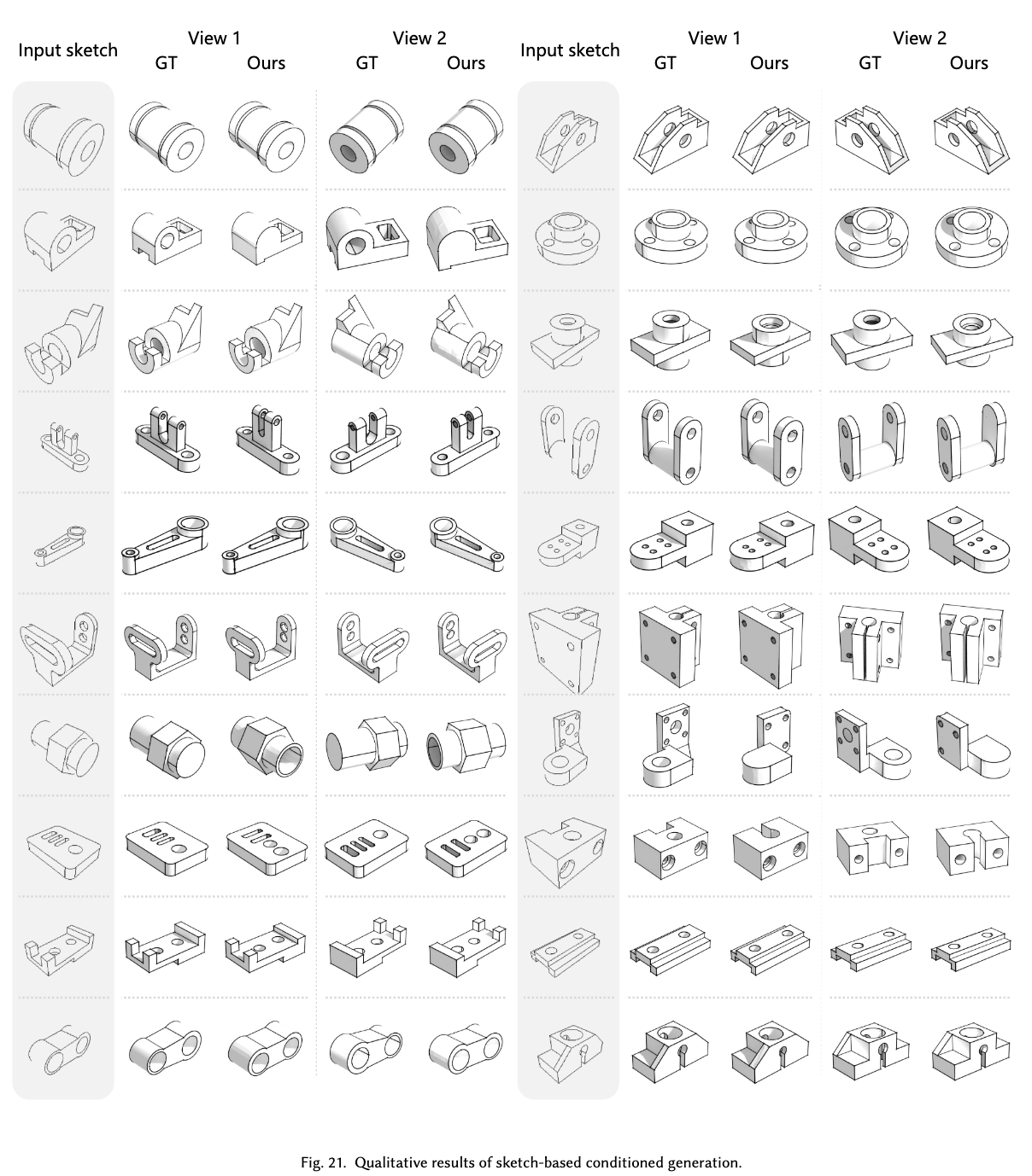
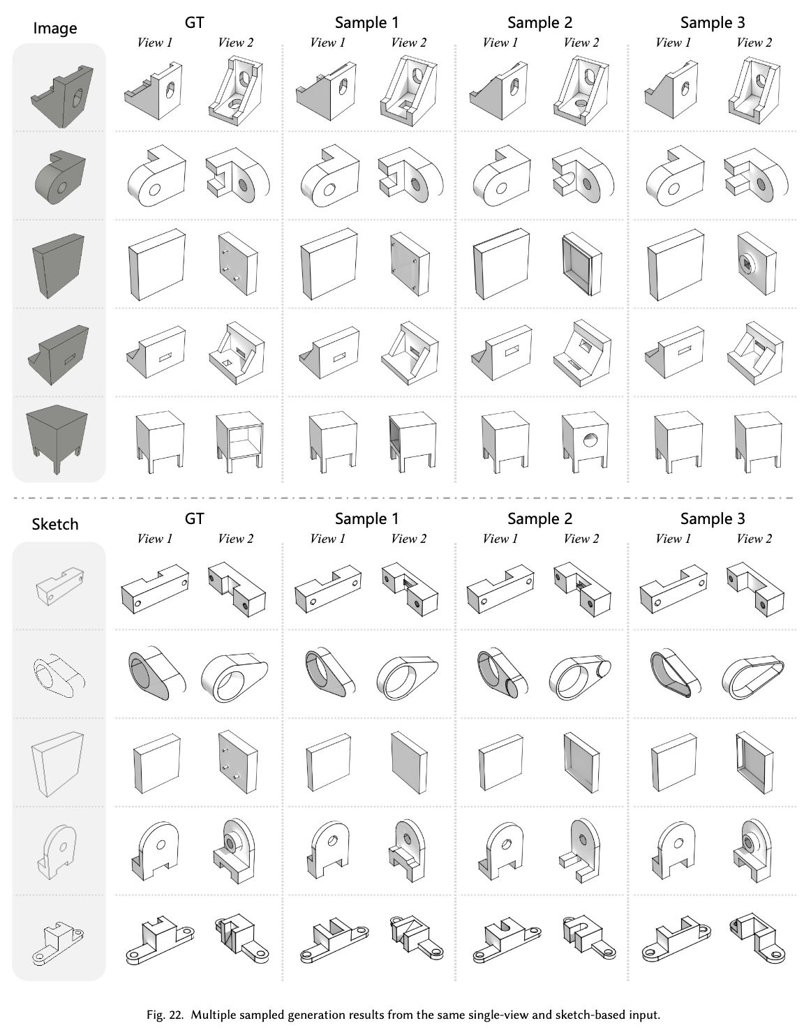
• Conditional Generation

  • 정량적 결과

    

    

    

  • 정성적 결과

    

    

    

    

    

    

• 실패 사례

  

  

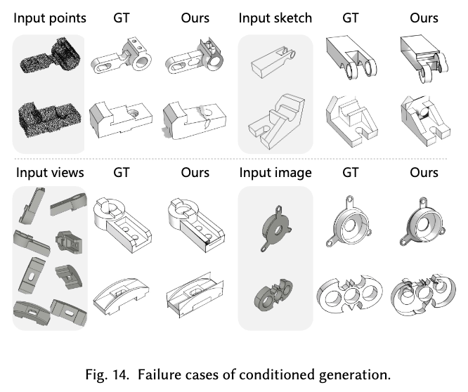
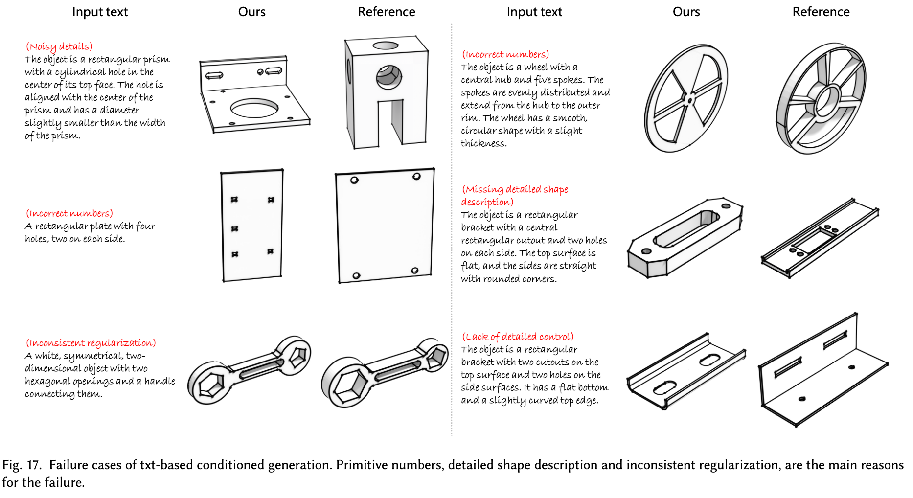
• Out-of-Distribution 사례

  

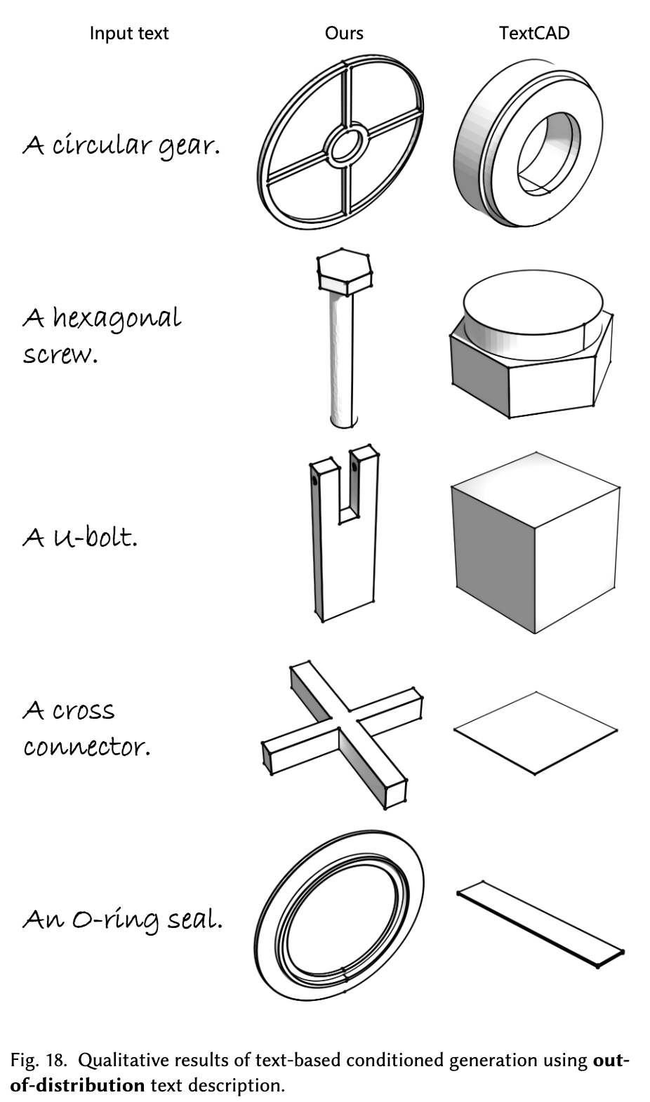
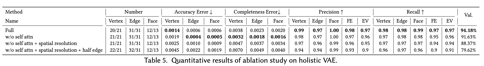
• Ablation Studies

  • SA / SR / HE 유무에 따른 분석

    

  • 반복 횟수에 따른 비교
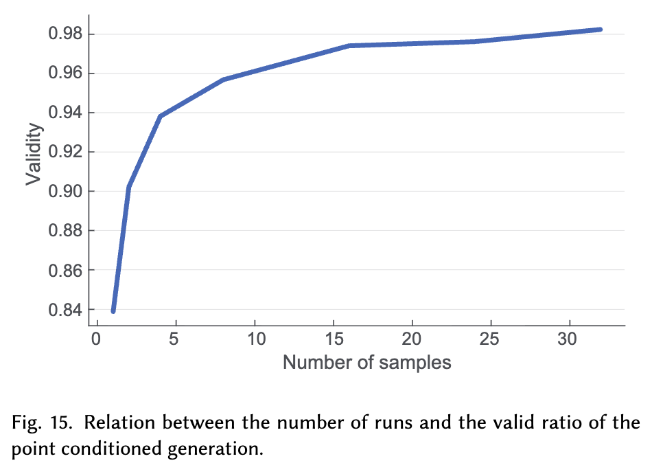