[DG][GM] EBTSA: ENERGY-BASED TEST SAMPLE ADAPTATION FOR DOMAIN GENERALIZATION
[DG][GM] EBTSA: ENERGY-BASED TEST SAMPLE ADAPTATION FOR DOMAIN GENERALIZATION
- paper: https://arxiv.org/pdf/2302.11215.pdf
- github: https://github.com/zzzx1224/EBTSA-ICLR2023 (깡통)
- ICLR 2023 accepted (인용수: 10회, ‘24-01-16 기준)
- downstream task: DG for CLS
1. Motivation
-
Deploy된 환경에서 single sample로 model parameter를 adaptation하는 것은 제한된 정보를 제공하므로 domain gap이 큰 상황에서는 문제를 야기할 수 있음
-
차라리 target domain sample을 source data로 adaptation하면 source data로 학습된 모델이 성능을 발휘할 수 있지 않을까?
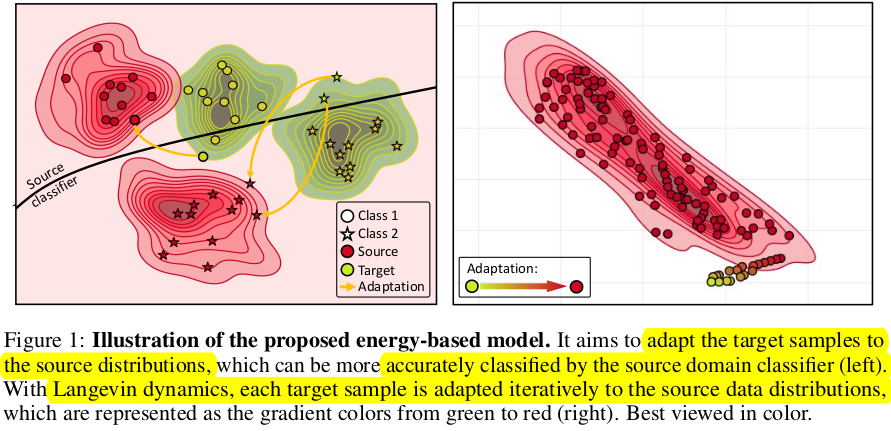
- (초록색) target sample들의 t-SNE cluster 분포 (2-class)
- (빨간색) source sample들의 t-SNE cluster 분포 (2-class)
-
최근 각광받는 Energy-based model로 complex data distribution을 modeling해보자! $\to$ Langevin Dynamics
2. Contribution
-
Energy-based Model을 활용하여 unseen target sample을 souce-trained model에 adaptation하는 EBTSA (Energy-Based Target Sample Adaptation)를 제안함
-
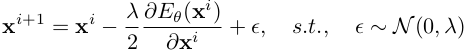
Iteratively Langevin dynamics를 활용하여 sample의 energy를 minimization하는 방향으로 학습 수행

- x$^{i+1}$: i+1번째 step의 adapted target sample
- x$^{i}$: i번째 step의 adapted target sample
- $\theta$: Energy based model parameter (neural network)
- $E_{\theta}$: Energy Function $ \in \mathbb{R}^D \to \mathbb{R}$
- $\lambda$: hyper-parameter
$\to$ No fine-tuning (adaptation) required!
-
Categorical 정보를 잃지 않고자, categorical prototype latent vector z를 함께 활용하여 sample adapation 수행

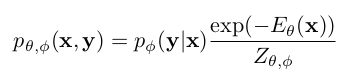
- $p_{\theta, \phi}$(x, y): probability score
- x, y, z: input image feature, label space, categorical latent variable
- $\phi$: classification model parameter
- $Z_{\theta, \phi}$: $=\int exp(-E_{\theta}(x))$ , intractable partition function
- 어떻게 z를 얻는지? classification model에 variational inference롤 통해 계산함
- inference time에는 어떻게? unseen target을 source domain 각각으로 adaptation시킨 ensemble결과를 활용 (multi-source)
-
3. Energy Based Test Sample Adaptation
- unseen target sample을 모방하고자, 서로 다른 source domain sample을 다른 source domain으로 adaptation 수행
3.1. Energy-based model
-
probability distribution을 Energy로 modeling
\[p_{\theta}=\frac{exp(-E_{\theta}(x))}{Z_{\theta}}\] -
위 분모 term이 intractable하므로, log-likelhood probability $logp_{\theta}(x)=-E_{\theta}(x)-logZ_{\theta}$를 maximize 수행하는 방식으로 대체

- 1st term : data distribution ($p_d(x)$). 에너지를 최소화 해야 maximum likelyhood estimate 할 수 있음
- 2nd term : model distribution ($p_d(x)$). 에너지를 최대화 해야 maximum likelyhood estimate 할 수 있음
- Model $p_{\theta}$를 approximate하는 가장 Naive 한 방법은 MCMC $\to$ Stochatic Gradient Langevin Dynmaics르 대체
-
Stochatic Gradient Langevin Dynmaics로 대체
-
$logp_{\theta}(x)=-E_{\theta}(x)-logZ_{\theta}$를 최대화 하는 또 다른 방식 $\to$ KL divergence of $\mathbb{D}{KL}(p_d(x|p{\theta}(x)))$을 최소화
-
minimizing contrastive divergence
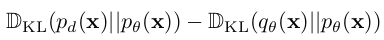
- $q_{\theta}(x)=\Pi_{\theta}^tp_d(x)$: t seqeuential MCMC starting from p(x)
-
위 식은 아래 식을 최소화함으로 구현 가능

3.2. Energy Based Test Sample Adaptation
- intial value : uniform distribution $\to$ target sample로 대체
- target sample을 source sample로 adaptation하는게 목표
-
-
Overall diagram
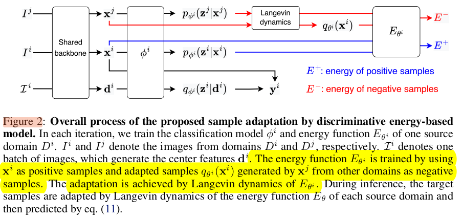
- x$^i$: i번째 source domain에 속한 sample
- x^j: j번째 source domain에 속한 sample
- Energy based model은 source domain별로 존재하며, real sample from i domain은 positive, adapted sample from j domain은 negative로 contrastive 학습
Discimiative Energy-based Model
-
$p_{\theta, \phi}$ (x, y): classification model($\theta$)과 energy based model$\phi$로 구성됨
- x: image I의 backbone featuer
- y: label space vector
-
contrastive divergence loss를 사용하여 최소화 (Eq. 6)

- 정리하면
- $q_{\theta}(x)=\Pi_{\theta}^tp_d(x)$: t seqeuential MCMC starting from p(x)
Label-preserving adaptation with categorical latent variable
-
Navie한 Langevin Dynamics는 sampling은 input feature X space에서만 수행되고, start point과 독립적으로 random sampling하므로 categorical 정보가 없음
-
label-preserving adaptation을 위해 categorical latent vector z를 도입 X space $\to$ X $\times$ Z space 에서 sampling

- $\phi$: classification model의 parameter로, x, z를 예측함
- $\theta$: z given x에 대한 maixmum probability를 modeling하는데 사용되는 energy function network parameter
- z는 fixed되어 사용
-
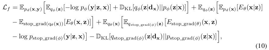
lower bound of log-likelyhood $log p_{\theta, \phi}$(x, y) (Eq. 9)

-
위 식 (9)를 (6)에 대입하여 정리하면
-
z는 variational inference로 예측함 (q(z* d$_x$)) - d$_x$: category x로 예측된 average representation of samples on source domain $\to$ class prototype 같은 느낌
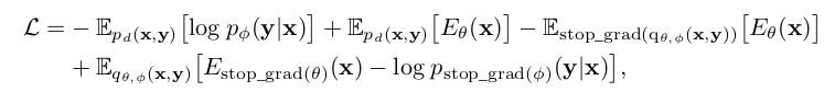
- 1st term: source data로 classification model $\phi$를 학습
- 2nd term: source data로 energy-based model $\theta$를 학습
- 3rd term: adapted sampe에 대해 adaptation 과정을 학습시킴
-
Ensemble Inference
-
S개의 source energy, classifier model의 ensemble 결과를 활용
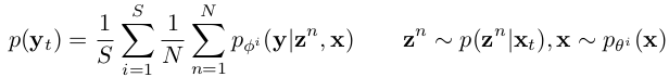
- z$^n$: n번째 sample
-
p(z$^n$ x$_t$): target sample feature에 대해 n번째 sample의 prior probability distribution - S: source domain sample의 갯수wfa
4. Experiments
-
vs. SOTA
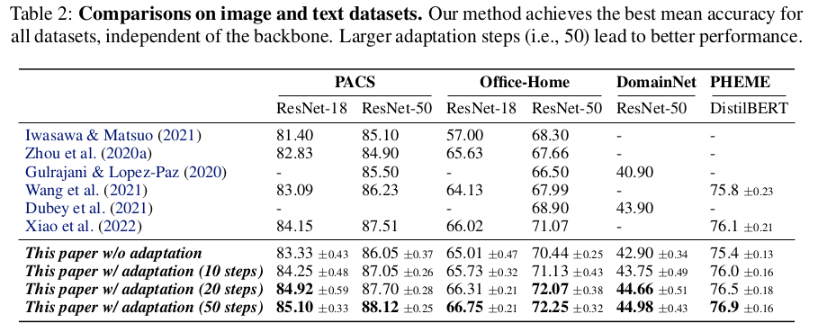
-
iterative adation의 유효성
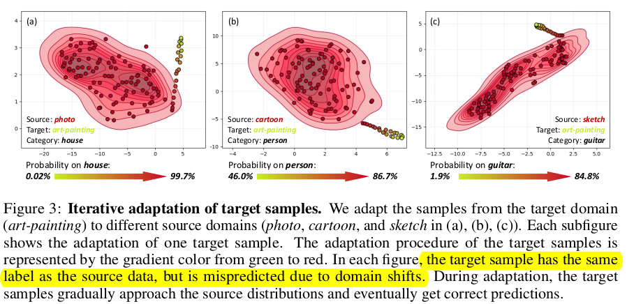
- 위 실험에서 보여지는 point들은 모두 source/target 은 동일 class임
-
Lagevin dynamic step number에 따른 ablation study
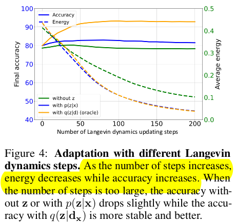
-
(주황색) 실제 target domain의 class prototype을 적용한 경우
-
(파랑색) single target sample에 대해 class prototype (d$_x$)을 적용한 경우
-
(초록색) z latent vector를 적용하지 않은 경우
$\to$ (주황색)vs. (파랑색) energy는 minimization하는 방향으로 sample을 adaptation하기 때문에 oracle과 같이 떨어짐. 하지만, single sample만 사용하여 target sample의 category prototype 을 정밀하게 예측하지 못하므로, accuracy는 차이가 나는 것임
$\to$ (파랑색) vs. (초록색) z 유무에 따른 energy / accuracy 비교. z를 사용하는게 안정적이며, accuracy로 향상시킴. 즉, adaptation이 잘 됨을 의미함
$\to$ (파랑색) step이 너무 커지면, energy는 감소하지만, accuracy가 줄어듦. 이는 sample의 category prototype 을 정밀하게 예측하지 못하므로, accuracy는 떨어짐
-